Visualized: Microservices as the Upper Bound for Monolith Availability

Switch to Korean

viewof p = Inputs.range([0.01, 0.99], {step: 0.01, value: 0.5, label: "p"});
viewof n = Inputs.range([1, 100], {step: 1, value: 5, label: "n"});

function join(p, n) {
  return Math.pow(p, n);
}
function split(p, m) {
  return 1 - Math.pow(1 - p, m);
}

y1s = (() => {
  const ys = [];
  for (let i = 1; i <= 100; i++) {
    ys.push({
      m: i,
      y: join(split(p, i), n),
      label: "ScaleOutMicroservice",
    });
  }
  return ys;
})();

y2s = (() => {
  const ys = [];
  for (let i = 1; i <= 100; i++) {
    ys.push({
      m: i,
      y: split(join(p, n), i),
      label: "ScaleOutMonolith",
    });
  }
  return ys;
})();

Plot.plot({
  grid: true,
  color: {legend: true, scheme: "BuRd"},
  x: {label: "m"},
  y: {label: "Combined Availability", domain: [0, 1]},
  marks: [
    Plot.areaY(y1s.concat(y2s), {y1: "y", x: "m", fill: "label", fillOpacity: 0.5}),
    Plot.tip(y1s, Plot.pointerX({x: "m", y: "y", fill: "darkgray", title: (d) => `${d.label}(${p}, ${d.m}, ${n})\n${d.y}`})),
    Plot.tip(y2s, Plot.pointerX({x: "m", y: "y", fill: "darkgray", title: (d) => `${d.label}(${p}, ${d.m}, ${n})\n${d.y}`})),
  ],
  style: "background: inherit;",
});

Figure 1: The Observable Benefits of Horizontal Scaling (Scale-Out) of Microservices

Comparisons Through Examples of Monoliths and Microservices

Shared Source Code of Monoliths and Microservices

According to web developer Krtalić Rusendić (2022), a single program is considered a monolithic architecture, while implementing the same program as multiple programs is called microservice architecture, or MSA.

A monolithic program is composed of classes and methods, or modules and functions (Krtalić Rusendić 2022). If classes and methods are implemented as a microservice program, they become services and APIs (Krtalić Rusendić 2022). Netflix is well-known for its use of microservices, and they have also developed a testing tool called Chaos Monkey (Krtalić Rusendić 2022).

Krtalić Rusendić (2022) presents an engaging visualization of the differences between monoliths and microservices. However, the claim by Krtalić Rusendić (2022) that the availability of the program he came up with is \(50\%\) for monolith and \(25\%\) for microservice was not about the source code. Failures caused by defects in the source code should result in a \(25\%\) availability regardless of whether the deployment is monolith (one program) or microservice (two or more programs). For example, if you run a source code that outputs only when the sum of two random numbers (0 or 1) is 0, the availability is \(25\%\) whether the random generation is sequential or parallel, or whether the deployment is monolith or microservice. When deploying this program as microservice instead of a monolith, the single point of failure (SPOF) is not increased to two; even in a monolith, there are two single points of failure (SPOFs) due to dependencies between results.

Partial Benefits of Source Code of Microservices

Designing a system as a microservice can be advantageous even if it is deployed later as a monolith. In the aforementioned source code, if one decides to produce not just the sum of two results but also an intermediate output of the first result only when it is 0, the availability becomes \(50\%\) because the output is independent of the second result. In this case, the single point of failure (SPOF) is only the first result, and there is no need to unnecessarily depend on the second result, either, and increase the single point of failure (SPOF) to two, ending up with the reduced availability of \(25\%\). Thus, considering partial availability or resilience in the design stage keeps the number of single points of failure (SPOFs) from being unnecessarily increased, even if deployed as a monolith.

An Analogy of NAND Flash Memory To Understand Trade-Offs Between Monoliths and Microservices

Beyond the source code, it is probable that microservices have more costs compared to monoliths (see Krtalić Rusendić 2022). If the hardware on which the two units of example source code depend is a single unit, and the availability external to source code is presumably \(50\%\), then if each source code depends on a different hardware unit, the availability could virtually drop to \(25\%\) due to the asynchronous operations of independent hardwares.

However, the significant costs of monoliths compared to microservices should not be overlooked, either. If two units of example source code depend on two hardware units in total, and the availability independent of source code is given \(25\%\), then consolidating them to depend on a single hardware component may reduce availability further to \(12.5\%\) due to resource contention. For example, NAND Flash memory faces similar opportunity costs in terms of quality (performance, durability, reliability, or etc.) depending on whether its type is single-level cell (SLC), multi-level cell (MLC), triple-level cell (TLC), or quad-level cell (QLC) (see Lee 2018). Generally, single-level cell (SLC) flash is more expensive and performs better than quad-level cell (QLC) flash. In other words, monoliths may suffer from disadvantages similar to those of quad-level cell (QLC) flash.

The Visualized Trade-Offs Between Monoliths and Microservices

Figure 3 explains this difficulty of comparison regarding hardware. The availability of the same source code is shared as equal in between both of the deployment methods, microservices and monoliths, as described earlier.

flowchart TB

    subgraph monolith[Monolith: 2/4 * 1/3]

        sc2a-.-hu3c1
        sc2b-.-hu3c2

        subgraph Source Code

        sc2a--->sc2b

        sc2a[A]
        sc2b[B]
        end
        
        subgraph Hardware Unit 1

        %% hu3c1 e1@--> hu3c2
        hu3c1 --> hu3c2

        hu3c1[Consumed
                0]:::consumed
        hu3c2[Consumed
                0]:::consumed
        hu3u1[Unavailable
                1/2]:::unavailable
        hu3u2[Unavailable
                1/2]:::unavailable
        end
        
    end

    subgraph microservice[Microservice: 2/4 * 2/4]

        sc1a-.-hu1c1
        sc1b-.-hu2c1

        %% hu1c1 e2@--> lb1 e3@--> hu2c1
        hu1c1 --> lb1 --> hu2c1

        lb1[Optional
                API Gateway]:::api-gateway

        subgraph Hardware Unit 2
        hu2c1[Consumed
                0]:::consumed
        hu2a2[Available
                1/3]:::available
        hu2u1[Unavailable
                1/3]:::unavailable
        hu2u2[Unavailable
                1/3]:::unavailable
        end

        subgraph Hardware Unit 1
        hu1c1[Consumed
                0]:::consumed
        hu1a2[Available
                1/3]:::available
        hu1u1[Unavailable
                1/3]:::unavailable
        hu1u2[Unavailable
                1/3]:::unavailable
        end

        subgraph Source Code
        sc1a--->sc1b
        sc1a[A]
        sc1b[B]
        end

    end

    subgraph Initial Hardware Unit
    ihua1[Available
            1/4]:::available
    ihua2[Available
            1/4]:::available
    ihuu1[Unavailable
            1/4]:::unavailable
    ihuu2[Unavailable
            1/4]:::unavailable
    end

classDef consumed fill:#000,color:#f96
classDef available fill:#0f0
classDef unavailable fill:#f00,color:#fff
classDef api-gateway fill:#f96

%% edge classes not supported in v11.2.0
%% classDef animate stroke:#f96,stroke-dasharray: 9,stroke-dashoffset: 900,animation: dash 25s linear infinite;
%% class e1 animate
%% class e2 animate
%% class e3 animate
linkStyle 3,6,7 stroke:#f96,stroke-dasharray: 9,stroke-dashoffset: 900,animation: dash 25s linear infinite;

Figure 2: A diagram of comparison between microservices and monoliths concerning hardware.

It might seem that \(\frac 2 4 = 50\%\) in the monolith gets lower to \(\frac 2 4 \times \frac 2 4 = 25\%\) in the microservice because of asynchronous hardwares. However, the joint probability of availability is dependent on the more granular availabilities of the resource units inside the hardware units. It follows that \(\frac 2 4 \times \frac 2 4 = 25\%\) in the microservice may even lower to \(\frac 2 4 \times \frac 1 3 = \frac 1 6 \approx 17.67\%\) in the monolith since the available resource units in the monolith hardware get contended as more as each one of them is consumed; from \(\frac 2 4\), to \(\frac 1 3\), and to \(\frac 0 2\).

Nevertheless, the availability in the microservice could still decrease relying on the availability of the optional api gateway and that of the yellow routing arrows. It can be simper when we consider the probabillities the yellow edges denote as included in the following affected resource units. If only the availability of the following unit shrinks from \(\frac 2 4\) further to less than \(\frac 1 3\), monolith might beat the microservice.

The problem is that the internal availabilities of hardware units are not fixed as independent constants but conditional and interdependent on the amount of consumption. Therefore, in the following paragraphs, we will compare availability only from the perspective of the source code.

The Visualized Benefits of Horizontal Scaling (Scale-Out) of Microservices

Horizontal scaling (scale-out) is a strategy to remove single points of failure (SPOFs) and increase availability. In reviewing the analysis of Krtalić Rusendić (2022), it appears that two available states of microservices displayed in Figure 3 have been omitted out of 16 possible states, leading to slight miscalculations of the availability as \(\frac 7 {14} = 50\%\). Although the original calculation was conducted regardless of source code and the other availability of \(75\%\) for the horizontally scaled (scaled-out) monolith turns out as uncertain according to the previous explanation about hardware, we could still gain insights from the beautifully animated diagrams and discuss further about source code as well.

Figure 3: The Two Available States of Microservices in Horizontal Scaling (Scale-Out) Krtalić Rusendić (2022) Omitted

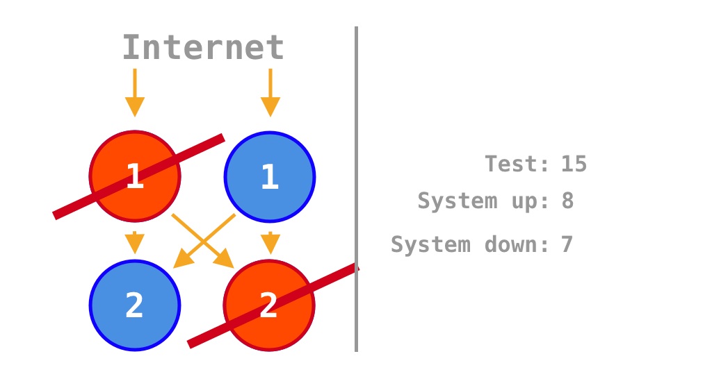
Just as the example source code can have four states based on two operations and calculates availability as \(\frac 1 4 = 25\%\), since \[2^2 = 4,\]

for four source code operations, there are not 14 states in total as listed by Krtalić Rusendić (2022) but 16 states when including the two omitted ones:

\[2^4 = 16.\]

If each of the two units of source code is scaled out by a factor of two, the original two single points of failure (SPOFs) are removed, and availability increases from the original \(\frac 1 4 = 25\%\) (for two units of source code) to

\[\frac 9 {16} = 56.25\%.\]

The \(\frac 9 {16} = 56.25\%\) differs somewhat from the \(\frac 7 {14} = 50\%\) calculated by Krtalić Rusendić (2022).

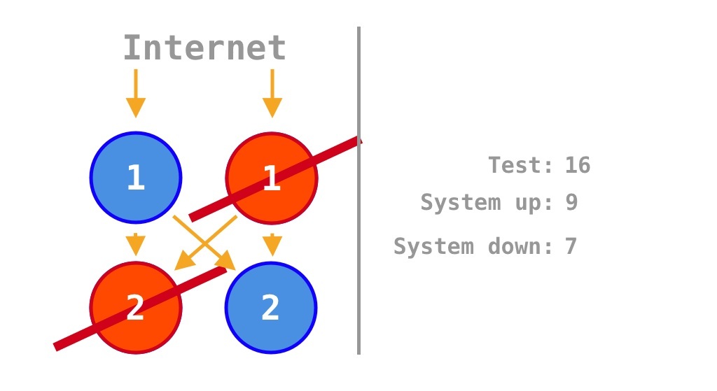
On the other hand, if the single points of failure (SPOFs) of a single monolith program are removed by scaling out the original program by a factor of two, the internal dependency between the two units of source code in the single program is maintained, but there is no external dependency between the two programs. Thus, the two yellow arrows in the center of Figure 3 are absent in Figure 4. Therefore, the two available states in Figure 3 become failure states in Figure 4, and the availability increases from \(\frac 1 4 = 25\%\) for a single program to

Figure 4: Horizontal scaling (scale-out) of Monoliths: 16 states

\[\frac 7 {16} = 43.75\%.\]

The \(\frac 7 {16} = 43.75\%\) differs somewhat from the \(\frac 3 4 = 75\%\) calculated by Krtalić Rusendić (2022). This is because, instead of scaling out a single program by a factor of four (to four instances), scaling out by a factor of two makes more sense for a rigorous comparison considering internal dependencies in the source code.

To summarize, from the perspective of the source code, the availability of a horizontally scaled (scaled-out) monolith (\(43.75\%\)) is better than the original \(25\%\), but it is still worse than that of a horizontally scaled (scaled-out) microservice (\(56.25\%\)). This represents a notable divergence from the interpretation offered by Krtalić Rusendić (2022).

Comparisons Through Formulae Between Monoliths and Microservices

Two Special Formulae Representing Shared Source Code of Monoliths and Microservices

Generally, when there are no external factors except source code, if \(n\) microservices with independent availability \(0 \leq p \leq 1\) are fully connected and depend on each other, they have \(n\) single points of failure (SPOFs). Therefore, their availability is the same whether deployed as microservices or monoliths:

\[\text{Join}(p, n) = p^n. \tag{1}\]

Since \(0 \leq p \leq 1\), this value decreases monotonically as \(n\) increases.

On the other hand, if \(m\) components are independent, they have no single points of failure (SPOFs), and their availability is the same whether deployed as microservices or monoliths:

\[\text{Split}(p, m) = 1 - (1 - p)^m. \tag{2}\]

This value increases monotonically as \(m\) increases, because \(0 \leq 1 - p \leq 1\) leads to \((1- p)^m\) decreasing monotonically.

A Formula Representing Combined Availability of Horizontal Scaling (Scale-Out) of Microservices

When there are no external factors other than source code, if each of \(n\) microservices with independent availability \(0 \leq p \leq 1\) is scaled out horizontally by a factor of \(m\), each group of \(m\) has no single points of failure (SPOFs) and its availability is \(\text{Split}(p, m) = 1 - (1 - p)^m\). If \(n\) groups of \(m\) are fully connected and depend on each other as \(n\) single points of failure (SPOFs), the combined availability is

\[ \begin{align} \text{ScaleOut}_{\text{Microservice}}(p, n, m) & = \text{Join}(\text{Split}(p, m), n)\\ & = \text{Join}(1 - (1 - p)^m, n)\\ & = (1 - (1 - p)^m)^n. \end{align} \tag{3}\]

This matches the availability in Figure 3:

\[ \begin{align} \text{ScaleOut}_{\text{Microservice}}(\frac 1 2, 2, 2) & = \text{Join}(\text{Split}(\frac 1 2, 2), 2)\\ & = \text{Join}(1 - (1 - \frac 1 2)^2, 2)\\ & = \text{Join}(1 - (\frac 1 2)^2, 2)\\ & = \text{Join}(1 - \frac 1 4, 2)\\ & = \text{Join}(\frac 3 4, 2)\\ & = (\frac 3 4)^2\\ & = \frac 9 {16}\\ & = 56.25\%. \end{align} \]

A Formula Representing Combined Availability of Horizontal Scaling (Scale-Out) of Monoliths

When there are no external factors, if \(n\) microservices with independent availability \(0 \leq p \leq 1\) are fully connected and depend on each other as \(n\) single points of failure (SPOFs), their availability when deployed as a monolith is \(\text{Join}(p, n) = p^n\). If the \(n\) components are scaled out horizontally by a factor of \(m\) to remove single points of failure (SPOFs), the availability is

\[ \begin{align} \text{ScaleOut}_{\text{Monolith}}(p, n, m) & = \text{Split}(\text{Join}(p, n), m)\\ & = \text{Split}(p^n, m)\\ & = 1 - (1 - p^n)^m. \end{align} \tag{4}\]

This matches the availability in Figure 4:

\[ \begin{align} \text{ScaleOut}_{\text{Monolith}}(\frac 1 2, 2, 2) & = \text{Split}(\text{Join}(\frac 1 2, 2), 2)\\ & = \text{Split}((\frac 1 2)^2, 2)\\ & = \text{Split}(\frac 1 4, 2)\\ & = 1 - (1 - \frac 1 4)^2\\ & = 1 - (\frac 3 4)^2\\ & = 1 - \frac 9 {16}\\ & = \frac 7 {16}\\ & = 43.75\%. \end{align} \]

The Inequality Representing the Benefits of Horizontal Scaling (Scale-Out) of Microservices

The following can be proven (Sil 2016):

\[(1 - (1 - p)^m)^n + (1 - p^n)^m \geq 1. \tag{5}\]

Therefore,

\[ \begin{align} (1 - (1 - p)^m)^n & \geq 1 - (1 - p^n)^m\\ \text{Join}(\text{Split}(p, m), n) & \geq \text{Split}(\text{Join}(p, n), m)\\ \\ \therefore \text{ScaleOut}_{\text{Microservice}}(p, n, m) & \geq \text{ScaleOut}_{\text{Monolith}}(p, n, m). \end{align} \tag{6}\]

The Observable Benefits of Horizontal Scaling (Scale-Out) of Microservices

In addition to the inequality of Equation 6, but the visualization in Figure 1 also demonstrates that the gap between \(\text{ScaleOut}_{\text{Microservice}}(p, n, m)\) and \(\text{ScaleOut}_{\text{Monolith}}(p, n, m)\) widens rapidly as \(p\) decreases or \(n\) increases, even as the factor of horizontally scaling (scale-out) \(m\) grows.

Conclusion

In conclusion, when there are no external factors besides source code, uniformly applying \(m\)-fold horizontal scaling (scale-out) allows microservices to internally remove single points of failure (SPOFs), resulting in higher combined availability than monoliths, which remove single points of failure (SPOFs) externally. Designing a system as a microservice in advance also offers the advantage of partial availability or resilience even when later deployed as a monolith. However, apart from source code, both resource contention in monoliths and the increased dependency of microservices on diverse resources must be carefully weighed and balanced.

References

Krtalić Rusendić, Stanko. 2022. “"Having a Monolith Is a Single Point of Failure".” September 30, 2022. https://stanko.io/having-a-monolith-is-a-single-point-of-failure-3cYdY3KZ7qHW.

Lee, Heeyeol. 2018. “[궁금한 반도체 WHY] 낸드플래시 메모리의 데이터 저장방식, 어떻게 다를까? SLC/MLC/TLC/QLC.” December 26, 2018. https://news.skhynix.co.kr/data-in-nand-flash-memory/.

Sil. 2016. “If \(p + q = 1\) Prove That for Any Natural \(n, m\) Following Is True: \((1 - p^n)^m + (1 - q^m)^n \ge 1\).” December 8, 2016. https://math.stackexchange.com/a/2049972.